What is PIV ( Particle Image Velocimetry )
Table of Contents
What is PIV
PIV stands for Particle Image Velocimetry, which is a flow visualization technique widely used in various fluid dynamics studies. PIV involves seeding particles into a fluid and illuminating them with a sheet of laser light twice in rapid succession. By analyzing two consecutive particle images captured at the same time as the illumination, PIV can measure not only the velocity magnitude but also the direction in both 2D and 3D space, as well as temporal data. It is a powerful tool for visualizing and quantifying fluid flow phenomena.
Basic principles of PIV
PIV, is a flow visualization technique widely used in various fluid dynamics studies. PIV involves seeding particles into a fluid and illuminating them with a sheet of laser light twice in rapid succession. By analyzing two consecutive particle images captured at the same time as the illumination, PIV can measure not only the velocity magnitude but also the direction in both 2D and 3D space, as well as temporal data. It is a powerful tool for visualizing and quantifying fluid flow phenomena.
The basic principle of PIV involves seeding small particles into the flow to be measured (seeding), and illuminating the measurement area of the resulting flow field with a laser light source such as a double-pulse YAG laser, which generates a sheet of light through a dedicated optical system. Then, two consecutive images are captured by a double shutter camera synchronized to the illumination timing. The double-pulse laser and double-shutter camera are synchronized to record two particle images with a very short time interval, typically less than 100 μs. In the analysis software, the displacement and velocity of each individual particle are calculated by identifying them within the acquired images.
There are various solutions for Particle Image Velocimetry (PIV) such as 2D-PIV which measures 2D velocity components in the plane illuminated by the laser light sheet, 3D-PIV which achieves simultaneous multipoint 3D measurement in the light sheet plane, time-resolved PIV which enables high-speed sampling from several kilohertz to several tens of kilohertz, confocal micro-PIV which enables 3D analysis of microfluidic flow distributions, probe-type PIV which integrates laser and camera in a probe without calibration, and shadowgraph PIV which captures flow conditions by combining shadowgraphy with PIV analysis of bubble flow. In this article, we will explain the principles of PIV, the algorithm for PIV analysis, and post-processing in detail.
PIV analysis procedure

- Introduce tracer particles into the flow field (wind tunnel or water tank) (seeding).
- Acquire images of the test object illuminated by bright lighting with two short exposures.
- Image analysis with various algorithms
- Acquisition of PIV data
- Post-processing as needed, such as removing false vectors
Seeding
Selecting tracer particles with an appropriate size for the measurement area is an important factor in determining the measurement accuracy when conducting PIV measurements. It is also necessary to consider contamination or health hazards related to wind tunnels or test objects and to perform proper seeding.
Image acquisition
To perform PIV analysis, particle images are acquired by illuminating the flow field twice with laser light and photographing with a camera. The technology of CCD and CMOS cameras has evolved, and since it is possible to acquire images at high speed and with low noise, analysis accuracy is improving.
Frame straddling
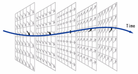
PIV typically requires two consecutive particle images with a very short time interval of less than 100 microseconds. The blue line above indicates the two camera exposures, while the green line indicates the two laser pulses. These laser pulses span the inter-frame time between the two camera exposures, a technique called "frame-straddling."
Frame-straddling techniques enable recording of two consecutive images with time intervals as short as 100 nanoseconds. Double-pulse lasers and double-shutter cameras are synchronized by a timing controller. Double-pulse lasers have two independent laser heads, enabling very short laser oscillations regardless of the duration of non-exposure time between the two frames of the double-shutter camera.
Optical system
To safely use high-output lasers, they are typically operated in the green light range around 532 nm. Fibers or arms are used to guide the laser to the flow field. The thickness of the illumination is adjusted using a sheet optics system. Adjusting the sheet thickness is crucial since the particle images used for analysis are obtained from the part of the sheet that is illuminated. In recent years, LED light sources have also been used for simple measurements instead of lasers, but a sheet optics system that matches the directionality of the LED element is required in this case. Selecting the optimal thickness for the test area is necessary, and the combination of lenses on the camera side is also an important factor that determines the analysis accuracy.
Analysis
Analysis is performed based on the obtained particle images to calculate trajectories and flow velocities. The technique of analyzing each individual particle is called PTV (Particle Tracking Velocimetry). In PIV, analysis is performed by dividing the particle images into search areas.
Evaluation of particle movement and velocity

After obtaining suitable images using frame straddling, the next step is PIV analysis. The images are divided into small search areas, typically 32x32 pixels (the search area is considered depending on the particle image). These small search areas are called interrogation windows.
Cross-correlation is applied to both images for these interrogation windows, obtaining a correlation surface for each interrogation window. The position of the interrogation windows in both images is the same (in standard FFT cross-correlation, the interrogation windows are shifted by advanced algorithms).
Then, peak detection and displacement evaluation are applied (using FFT cross-correlation), obtaining the dominant displacement in each interrogation window. By performing calibration beforehand, the pixel size in the flow (acquired image) and the time interval between the two images are known, so the velocity can be calculated. The pixel size in the acquired image is determined relatively easily by taking a scale photograph and inputting the value (the distance per pixel is measured using scales or targets).
The analysis algorithm is designed to be optimal depending on the scale and frequency of the subject being studied.
Analysis algorithm
There are various algorithms available for estimating motion. The PIV analysis algorithm of Seika Digital Image's Koncerto II adopts state-of-the-art deformation correlation developed by the German Aerospace Center (DLR), allowing for high-precision PIV analysis. Additionally, it is equipped with post-processing capabilities such as specialized time-series PIV algorithms (FD4), POD analysis, and vorticity visualization. The main analysis algorithms are described below.
Standard FFT cross-correlation
Basic displacement (velocity) evaluation method. It provides results similar to direct cross-correlation in a short computation time.
Standard Single-Pass Interrogation
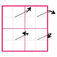
The figure shows a concept diagram of simple correlation. The displacement of a particle group within the same area (interrogation window: analysis window) of two images A and B is determined by cross-correlation analysis.
Multipul-Pass Interrrogation
The diagram below illustrates the concept of recursive correlation. First, the displacement of the particle group in the same area (interrogation window: analysis window) of the AB images is determined by correlation analysis using the simple correlation method. Then, the window in the second image is moved based on the correlation peak obtained from the AB images, and the analysis is repeated to improve the correlation value. By repeating this operation several times, the displacement approaches zero, and the analysis accuracy is improved.
←横スクロールでご覧いただけます→
 |
 |
 |
 |
 |
 |
 |
| STEP1 | STEP2 | STEP3 | STEP4 | STEP5 | STEP6 | STEP7 |
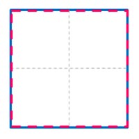
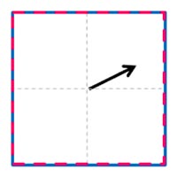
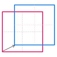
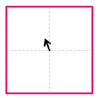
| Define window "a" in Image A (red box) and window "b" in Image B (blue box). | Take the correlation between window a and window b, and calculate the displacement to obtain Predictor 1. | Shift the window b in image B based on the displacement obtained from predictor 1, and define the shifted window as window b'. | Compute the correlation between window a and window b' to obtain predictor 2. | Shift window b' again using Predictor 2 and obtain window b" | Take the correlation between window a and window b", and obtain the displacement as predictor 3. | By repeating this process, the number of unmatched particles in the window decreases and the correlation value increases, improving the accuracy. The final endpoint of the last predictor is taken as the representative displacement in the initial grid. |
Multi-grid Interrogation
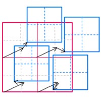
This is a concept diagram of hierarchical correlation. The window size is reduced with each iteration of the recursive correlation analysis. By maintaining a large maximum displacement, the window size can be reduced, thereby improving spatial resolution while maintaining velocity dynamic range. In addition, rotations within the initial window can also be accommodated.
←横スクロールでご覧いただけます→
|
|
|
 |
 |
 |
 |
| STEP1 | STEP2 | STEP3 | STEP4 | STEP5 | STEP6 | STEP7 |
| Define window a (red frame) in image A and window b (blue frame) in image B. | Calculate the correlation and displacement between window a (black frame) and window b (blue frame) and use it as the predictor 1 for the next step. | Shift the window b (blue frame) in the image B using Predictor 1, resulting in window b' | Divide both window a' and window b' into four smaller windows | Calculate the correlation in each 1/4 window and find the amount of movement and set it as predictor 2 (2-1, 2-2, 2-3, 2-4). The figure shows the case where there is a turn within the initial window | Shift windows B1, b2, b3, b4 in B image by four predictors 2 (2-1, 2-2, 2-3, 2-4) respectively | This iterative process can improve both accuracy and resolution. The displacement of each final window becomes the representative displacement for each grid resulting from the division. |
Image Deformation / Correlation
An algorithm for deforming images based on predictors obtained from multipath correlation or multigrid correlation. By recursively deforming images with sub-pixel accuracy, it is possible to almost completely eliminate errors caused by peak locking.
←Scroll horizontally to view more.→
 |
 |
 |
 |
 |
 |
| STEP1 | STEP2 | STEP3 | STEP4 | STEP5 | STEP6 |
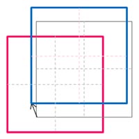
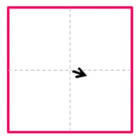
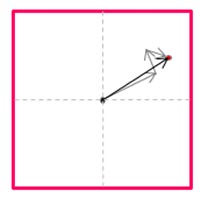
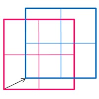
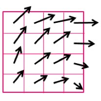
| You can obtain the displacement of particle groups in Window a of Image A and Window b of Image B (at the same position) using the standard correlation method. | Next, similarly determine the amount of movement of the particle group in the surrounding grid | Considering the analysis of the black central window, use the movement of particle groups in the surrounding grids as predictors to deform the B image. | If we schematically represent the image deformation, it would look like the following figure. The image is continuously deformed with each grid as a reference point. We will deform the eight points on the red-bordered grid in the figure into the blue-bordered configuration. | Calculate the correlation between window a in image A and window b in image B, obtain the displacement, and update the predictor. | This process can be repeated any number of times to improve accuracy. |
FD4 /Dedicated Algorithm for Time Resolved PIV
FD4 correlation is an algorithm developed for time-resolved PIV, enabling the analysis of temporal velocity fluctuation frequencies, turbulence, and high-precision spatiotemporal validation at each grid in PIV. In conventional 2D PIV analysis, error vectors generated during analysis are determined as correct or incorrect through spatial validation and are then interpolated through interpolation based on surrounding vector information. To perform accurate interpolation, surrounding vectors must be correct. However, in cases where error vectors occur continuously on a grid, interpolation may not be performed correctly. As the flow is continuous in time, time-resolved PIV enables improved accuracy even in such cases by analyzing along the time axis.
Effect of FD4 correlation
The top and bottom vector plots on the video represent instantaneous velocity vector fields at the same time.
At first glance, both plots appear to be accurately analyzed, but when viewed as a time series movie, it becomes clear that the vector plots without FD4 correlation (top) exhibit unnatural oscillations in the vicinity of the vortices.
On the other hand, the data with FD4 correlation applied (bottom) show that the velocity vectors at each time step are temporally continuous.
Analysis along the time axis
In time-resolved PIV analysis, the continuity between the preceding and succeeding data enables us to validate the velocity vectors by comparing them temporally. However, as the data are temporally close to each other, the preceding and succeeding data often contain erroneous vectors themselves, making it insufficient to compare only the adjacent data.
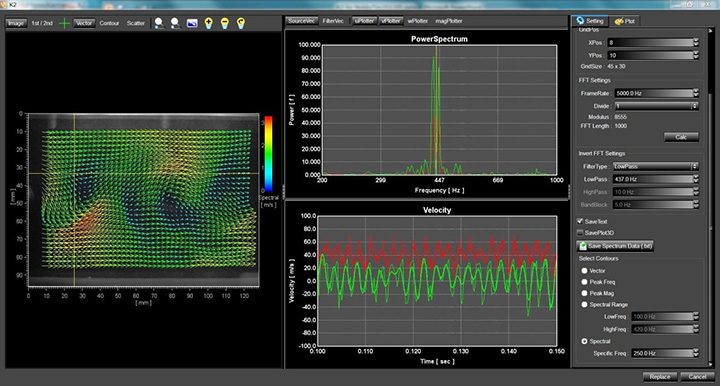
Therefore, FD4 correlation performs spectral analysis of the temporal velocity variations for each grid on the velocity map and calculates the theoretically optimal value for that specific time. The velocity variation spectrum obtained by Fourier transformation generally contains noise components on the high-frequency side, so a low-pass filter is applied to remove the noise components, and the data are transformed back to the time-domain using inverse Fourier transformation. When observing the velocity variation curve with velocity on the vertical axis and time on the horizontal axis, the erroneous vectors are observed as spike-like noise on the curve. The velocity variation curve filtered with a low-pass filter becomes a smooth curve with no spike noise. Based on this curve, a more reliable interpolated value can be obtained by calculating the theoretically optimal value for that specific time.
FD4 correlation achieves higher measurement accuracy by utilizing both spatial continuity in the conventional validation method and temporal continuity. It should be noted that the time-resolved PIV FD4 correlation algorithm was developed by the Miyauchi-Tanahashi Laboratory at Tokyo Institute of Technology and is a patented technology.
POD /Eigenorthogonal decomposition
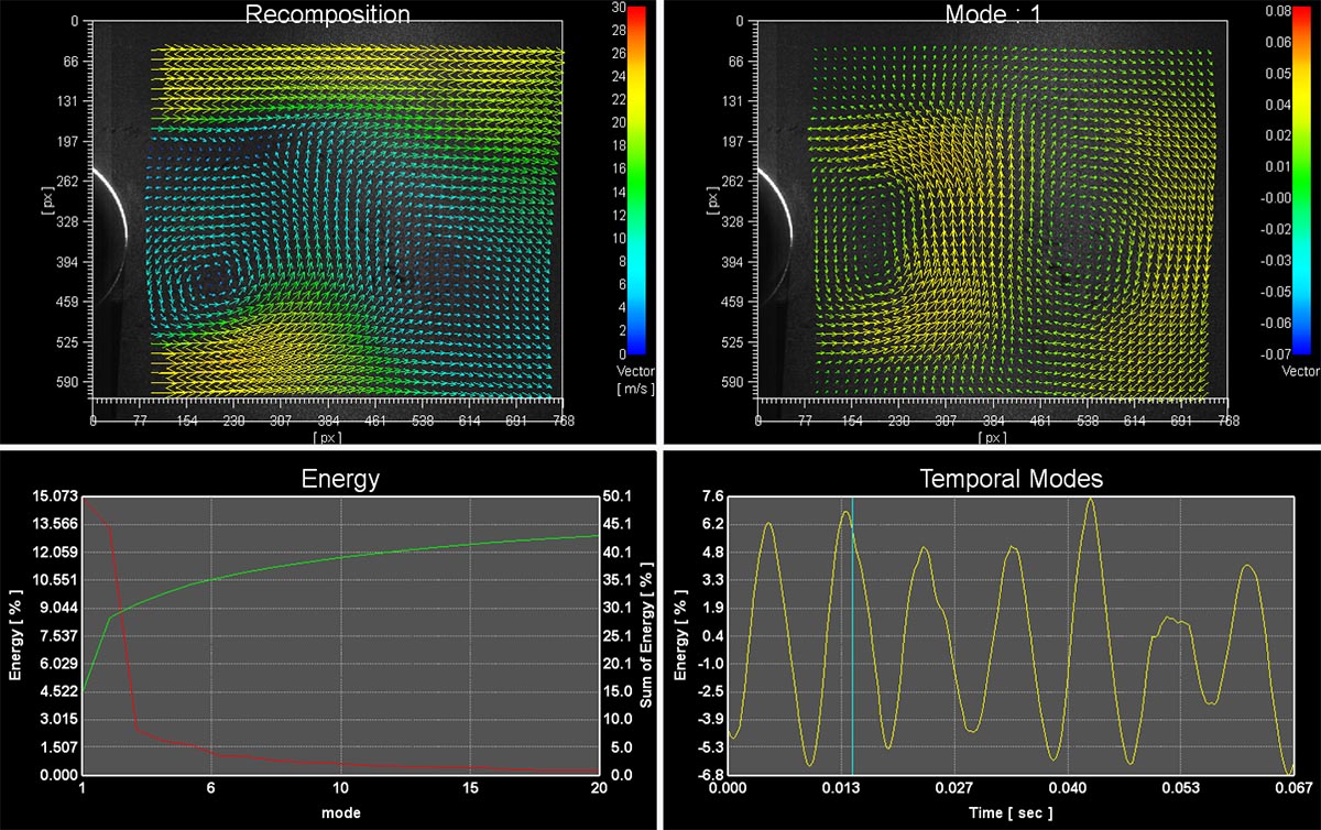
Proper Orthogonal Decomposition (POD) is a post-processing function used to extract important flow structures from velocity vector data obtained through PIV. In POD, the vector data (source vector) of the flow field obtained through PIV is decomposed into multiple modes (structures) in order of energy, and a simplified reconstruction vector is obtained that reflects only the energy that each mode contributes to the flow, by combining the source vector and any selected modes. This function is useful for comparing with CFD data and for flow control analysis, among other applications.